 五度妙笔
五度妙笔 API商城
API商城
 数据库
数据库Quantifying fairness in spatial predictive policing - Artificial Intelligence and Law
Abstract
Predictive policing leverages data-driven models to anticipate future criminal events and guide law enforcement strategies. However, concerns about algorithmic fairness have emerged, as these models risk perpetuating discrimination and inequities, particularly among vulnerable populations. While prior research has acknowledged the influence of disparities in crime reporting levels on these models, the extent of their impact on vulnerable populations remains insufficiently understood, posing a critical challenge in societies marked by high disparities. This study seeks to quantify the fairness of three prevalent density probability estimation models used in predictive security (Code available at https://tinyurl.com/Source-Code-GitHub). Specifically, it examines their capacity to distribute benefits impartially across diverse populations in various spatial contexts. Real-world theft data were employed to calibrate three distinct predictive models, followed by the quantification of model fairness through two different measurement approaches. These measurements assess disparities in the granting of model benefits between two geographical areas—one focusing on the average prediction error benefit and the other on the utilization of the model for resource allocation. Results suggest that the predictive security models studied may be fair for the prediction but unfair over the use of the model for patrol allocation, with a maximum difference between the means of groups of \(45\%\) and an average of these differences of \(12\%\). This highlights the nuanced nature of fairness considerations within predictive policing frameworks.
1 Introduction
Predictive security relies on data-driven models to anticipate future crime occurrences and inform security strategies (Hardyns and Rummens 2018). These systems typically analyze spatiotemporal incident data reported by citizens or compiled by law enforcement agencies to discern patterns and allocate resources effectively for crime prevention. Such insights are crucial for urban security planning across diverse contexts (Benbouzid 2019), from optimizing police patrols and security facility locations to implementing broader structural interventions, all of which significantly impact communities (Manning et al. 2018; Elzayn et al. 2018).
However, recent scrutiny of decision-supporting systems driven by data has underscored concerns about algorithmic fairness within predictive security systems (Akpinar et al. 2021). Studies have identified biases in these models that could disproportionately affect specific populations, exacerbating social inequalities (Wu et al. 2023). Consequently, despite their potential benefits, understanding and mitigating these biases is imperative for predictive security (Alikhademi et al. 2022).
Algorithmic fairness, an emerging area in artificial intelligence (AI), aims to address biases in machine learning (ML) models (Wang et al. 2023). It evaluates fairness by examining how benefits provided by models are distributed among different sub-populations using equity metrics (Wang et al. 2023; Caton and Haas 2024). A fair model ensures equitable treatment across various groups, a principle crucial for maintaining societal trust in these predictive systems. While fairness quantification strategies are well-established for individual-focused predictive models (Mittelstadt et al. 2023), applying these metrics to spatially-based predictive models, such as those used in predictive security, remains underexplored (Hardyns and Rummens 2018; Flynn et al. 2022). It is essential to emphasize that regardless of the predictive system’s nature, a fundamental requirement should be that demographic or socioeconomic factors do not influence predictions or decisions (Sacharidis et al. 2023).
This paper proposes a novel strategy for assessing spatially-based crime predictive systems, focusing on fairness both in prediction accuracy and resource allocation. Unlike previous work that primarily quantifies fairness in individual-focused models (Hung and Yen 2023), our approach aims to extend fairness quantification to the spatial predictive context commonly used in predictive security. Specifically, we introduce a profit function framework that integrates established fairness metrics to evaluate prediction accuracy and resource allocation fairness simultaneously (Hernandez-Boussard et al. 2023). By examining how predictive models influence decision-making processes, such as police patrol assignments, we hypothesize that fairness considerations may differ significantly in spatial predictive systems, highlighting the need for a comprehensive assessment framework.
In this study, we apply our proposed fairness evaluation strategy to two large cities, analyzing crime data across sub-populations defined by income and poverty levels. Our contributions include introducing a novel approach for fairness evaluation in spatially-based predictive security systems, quantifying equity in both prediction and resource allocation across diverse populations and geographic regions. By addressing prediction errors, bias reduction, and resource allocation fairness, this research aims to advance understanding and practices in fairness within predictive policing strategies.
2 Materials and methods
Figure 1 shows the scheme proposed to quantify fairness related to the prediction and the allocation of resources in spatial-based predictive security models. First, different areas of interest within the city are defined. These areas would be based, for instance, on socio-economic factors such as income, education, or any other factor of interest from the fairness perspective. These spatial segments define the groups for which fairness wants to be quantified. Then, data-based predictive crime models estimate maps with the expected intensity of the crime phenomenon (Sriram et al. 2024). Following, three different data-based models commonly used in the predictive crime domain were considered, namely, naive Kernel Density Estimation (naive), Time-Space Kernel Density Estimation (KDE), and Self-Exciting Point Process (SEPP), to study possible unfair results (Rosser and Cheng 2019). The predictive model outputs commonly inform strategies to allocate security-related resources (Zhu et al. 2022). In this case, these predictions served as input for a greedy optimization algorithm aimed at spatially allocating a set of patrols to regions with the highest predictive intensity of the crime, i.e., patrols are assigned to the so-called hotspots (Zhu et al. 2022).
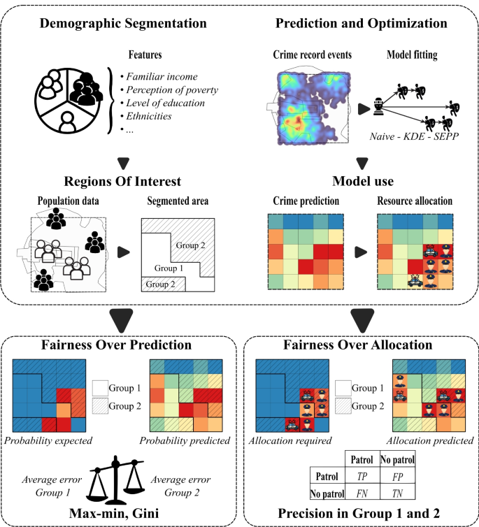
Proposed experimental schema for measuring fairness in prediction and resource allocation. First, the areas of interest are determined based on socioeconomic variables. Then, predictive models are trained to model expected event occurrences. These models also inform a resource allocation strategy. Prediction Fairness (PF) is calculated by considering how equitable the distribution of the prediction errors is for the different Groups. Resource Allocation Fairness (RAF) quantifies the differences in the precision of the assignation of patrols when a greedy optimization algorithm for resource allocation operates on the crime predictive maps
The fairness related to prediction quantifies how equitable the benefits provided by the predictive models are in the different areas of interest (Wang et al. 2023). In this case, high benefits link to small error rates for the predicted crime intensity. Complementary, fairness in resource allocation measures how well the predictions from the models help to assign resources (for instance, patrols) to control crime within the different spatial groups. In particular, how precise the assignation of these resources is within these areas.
2.1 Spatio-temporal crime incidents
Two fairness scenarios for two real crime settings were studied: Bogotá (Colombia) and Chicago (EEUU). The Bogotá data was provided by the Secretaria de Seguridad, Convivencia y Justicia de Bogotá (Colombia), a government agency responsible for security, coexistence, and justice in the city. 39.982 officially reported theft records from June 1, 2018, to December 31, 2019, were usedFootnote 1 . Events post-December 2019 were excluded due to notable behavioral changes stemming from COVID-19 quarantine policies (Ciotti et al. 2020). The selected records were from the largest populated city localities namely Chapinero, Santaf Fe, San Cristobal, Tunjuelito, Bosa, Kennedy, Fontibón, Engativá, Suba, Barrio Unidos, Teusaquillo, Los Mártires, Antonio Nariño, Puente Aranda, Candelaria and Rafael Uribe Uribe representing administrative divisions within Bogotá. Chicago’s crime data is available on its web portal (Department 2024). This portal reports crime events dating back to 2001 up to the present. The dataset studied includes thefts reported by citizens. For this study, 140.101 incidents related to thefts reported by citizens from June 1, 2022, to October 11, 2023, were used for analysis.
2.2 Groups of interest for fairness evaluation
A spatial segmentation was applied to define the groups of interest. The process of spatial segmentation relies on the observation that poverty perception and economic stratification have historically shaped people’s views on security (Lavrakas and Skogan 1984). Given the established correlations between high poverty perception and elevated crime rates (Morenoff et al. 2001), as well as the influence of economic stratification on spatial dynamics, this study explores whether these historical biases may be manifested in the predictive outputs of the models under scrutiny by evaluating fairness across these attributes. Panel (a) in Fig. 2 illustrates the proposed segmentation process. As observed, the work area is divided into groups of interest depending on variables related to the economic capacity.
For this, the spatial regions in Bogotá and Chicago were categorized into two groups: group 1 (\(G_1\)), composed by areas with a low perception of poverty and a high income, and group 2 (\(G_2\)), including areas with a high perception of poverty and a low income, i.e., potentially vulnerable or socially disadvantaged areas. The characteristic values for these categories were defined in Bogotá using official survey data from the region (Dimas Hoyos et al. 2015). The segmentation resulted from using the categorical description of the perception of poverty data (Dimas Hoyos et al. 2015). More specifically, high-income and medium perceptions were mapped to \(G_1\) and those perceived as in need to \(G_2\).
For defining the regions in Chicago, census data available in the data city portal was used (Bureau 2014). For this, the per-capita income was averaged across all community areas (Bureau 2014), and communities with values greater than this average were mapped to \(G_1\), while those with values less and equal to this value were to \(G_2\).
2.3 Areas of interest
Understanding potential biases in crime data requires careful consideration of the spatial and socioeconomic characteristics of urban environments. Previous research has shown that the presence of financial institutions, malls, and industrial zones can not only affect the true incidence of crime, but also adjust the presence of police and the likelihood of crime being reported (Rotaru et al. 2021; Akpinar et al. 2021). Such spatial heterogeneities can reinforce disparities in predictive policing systems if not properly accounted for.
To explore the extent of this phenomenon, we perform a spatial analysis of the datasets used for model training and evaluation. Specifically, we incorporate geospatial data on enterprise locations and central business districts. For Bogotá, Colombia, we use information from the public database “Datos Abiertos Bogotá”Footnote 2 (Cortes 2025), while for Chicago, USA, we use data from the “Chicago Data Portal”Footnote 3 (Levy 2025). This integration allows us to assess whether proximity to economic centers correlates with variations in reported crime rates, thereby introducing potential structural biases into crime prediction models (Xie et al. 2022; Villegas et al. 2023).
2.4 Predictive policing models
Three predictive policing models based on geographic data grids were explored: naive, KDE, and SEEP. These data-driven models are commonly employed to map crime hotspots (Cheng et al. 2021). They have proven effective for guiding constrained resource assignation, making them valuable for addressing security issues (Muggah and Tobón 2019).
2.4.1 Naive model
This model employs a Gaussian kernel to capture spatial relationships by assigning weights to spatial observations, emphasizing the proximity of events (Zambom and Dias 2012). Essentially, it assumes that when predicting information for a specific period, only events from that same period or with similar characteristics, such as the day of the week, in the historical data are considered. The model estimates the intensity of crime as follows:
where \(\lambda _{naive}(s)\) denotes the intensity for a specific spatial coordinate, \(s_i\) the spatial location of the i-th event, and \(K_s(\cdot )\) represents a Gaussian kernel summed over n events of a training period. This model results in high event intensity in areas for regions with a high historic rate of incidents.
2.4.2 KDE model
This model considers temporal distributions and spatial crime distribution. The model’s formulates the intensity of crime as follows:
here, \(\lambda _{KDE}(s,t)\) represents the expected intensity of crime at spatial location s and time t, where \(t_i\) denotes the temporal occurrence of the i-th event. The exponential function \(e^{-\beta (t-t_i)}\) captures the temporal component of crime occurrences by integrating the time difference between events and the prediction time, where \(\beta\) is a real number representing a decay exponent. This exponential function assigns more weight to events that are closer in time (Lee et al. 2017). The spatial component \(K_s(\cdot )\) is similarly calculated as the Gaussian kernel in the naive model. This model considers events occurring at the closest time-space, which may significantly influence prediction intensity. In this case, the model also accounted for daily predictions.
2.4.3 SEPP model
This model combines spatial and temporal interactions between events (Mohler et al. 2011). In addition, it accounts for self-excitation phenomena, where the occurrence of a crime raises the probability of additional events in proximity. In this model the intensity of crime is represented as follows:
where, \(\lambda _{seep}(s,t)\) represents the expected intensity of crime at spatial location s and time t, \(\mu (s)\) accounts for self-excitation from past events, calculated using a fixed bandwidth Gaussian KDE. The term \(\theta \omega e^{-\omega (t-t_i)}\) represents an inhomogeneous Poisson process where an event occurred at time \(t_i\), with \(\theta\) and \(\omega\) controlling the near-repeat behavior. The SEPP assumes that an event at a specific location and time increases the intensity of future events in the same area, irrespective of the events location.
2.5 Measuring fairness
Figure 2 illustrates the proposed fairness evaluation measurements: 1) fairness related to prediction and 2) fairness related to resource assignation. The prediction fairness quantifies how equitable the crime predictive models’ benefits are between groups. In this case, model benefits will link to lower error rates in prediction. Therefore, resource allocation fairness quantifies the differences in a model’s precision level when assigning resources to different groups.
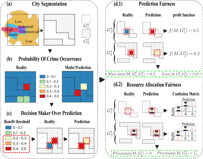
Proposed fairness pipeline in PF and RAF begins with defining the groups of interest for evaluation, followed by assessing the probability of crime occurrence in predictions and ground truth. Subsequently, the decision-maker restricts and selects analysis areas based on resource constraints. PF are then evaluated using profit functions, comparing result values in each group with the ground truth, e.g., in group 1, if prediction value is 0.5 and reality is 0, then \(f(M,G_{1}^*)=|0.5-0.0|=0.5\), and similarly, \(f(M,G_{2}^*)=|0.3-0.5|=0.2\). This allows calculation of PF metrics like Max-\(min(M,G_{1}^*,G_{2}^*)\)\(=|0.5-0.2|\)\(=0.3\) and \(Gini(M,G_{1}^*,G_{2}^*)=3\)\(\frac{|0.5-0.2|}{0.5+0.2}\)\(0.43\). Finally, RAF is calculated based on selected areas; if prediction is greater than 0, patrolling should occur, and similarly for the ground truth. With classifications of patrol and no patrol, a confusion matrix is constructed, and its precision values serve as fairness metrics, e.g., \(precision(M,G_{1}^*)=0\) and \(precision(M,G_{2}^*)=1\)
2.5.1 Prediction fairness (PF)
Prediction fairness involves a two-step process (Wang et al. 2023). The first step defines a benefit function, which determines the benefit allocated by the model to each group of interest. The second step involves comparing these benefits across each group using previously established fairness metrics such as Max-min and Gini. Through this comparison, we can assess the degree of fairness the model achieves in allocating benefits between different groups. These steps work as follow:
Benefit function. The benefit function for prediction is defined as the average of the absolute difference between the probability of occurrence predicted by the model and the ground truth intensity (Wang et al. 2023). The ground truth intensity results from normalizing the event count in each grid cell at a specific prediction time (day) with the total number of events occurring in this period, as illustrated in Panel (b) at Fig. 2. More specifically, the benefit function \(f(M, G)\) for the prediction provided by a model M on the complete set of cells within a group \(G\) is defined as:
$$f(M, G) = \frac{1}{|G|} \sum _{c \in G} |P_{M,c} - R_c|$$where \(P_{M,c}\) is the predicted crime intensity resulting from using the model M in the cell c, \(R_c\) is the ground truth value in the cell c and \(|G|\) represents the number cells conforming to the group \(G\). Importantly, this measure can be restricted for considering subsets \(G^* \subseteq G\), providing a mechanism for focusing on particular regions of interest within the group G by computing \(f(M, G^*)\). Panel (d.1) in Fig. 2 illustrates the profit prediction function computation focusing on two particular cells (red dashed cells) contained in \(G_1\) and \(G_2\), respectively. As observed, there is more average error in predictions for group \(G_1\) (0.5) than for \(G_2\). Importantly, in this case, the selected cells were determined by focusing on cells with high crime intensity in the predictions (Panel (c)). This approach provides a quantification for evaluating performance disparities between the two areas of interest, considering varying spatial coverage areas, which can differ significantly across different contexts or regions.
Metrics of PF. Based on the profit function, two measurements of disparity were computed to quantify the fairness of each model (Wang et al. 2023). The first measure was the Max-min, which calculates the absolute difference between the profits of each group. As only two groups exist, this measure corresponds to the absolute of the highest minus the lowest (Wang et al. 2023). This measurement characterizes absolute differences in intensity between the two groups. This metric was adapted for the cells of interest within each group and is defined as:
$$\text {Max-min}(M,G_{1}^*,G_{2}^*) = |f(M, G_{1}^*) - f(M,G_{2}^*)|.$$The second metric used is an adaptation of the Gini index for the context of fairness (Wang et al. 2023). In this case, the index calculates the distribution of the profits a model provides to different groups. The Gini fairness measure for cells of interest within the two groups was defined as:
$$\text {Gini}(M,G_{1}^*,G_{2}^*) = \frac{|f(M, G_{1}^*) - f(M,G_{2}^*)|}{f(M, G_{1}^*) + f(M,G_{2}^*)}.$$The Gini index measures the bias percentage in the model’s prediction errors. A Gini index close to zero suggests an equitable distribution of errors between the groups. In contrast, a high index and close to 1 implies a more biased distribution, indicating potential model bias toward specific groups regarding prediction errors. Panel (d.1) at Fig. 2 reports the Max-min and Gini PF metrics for a set of selected cells within the groups.
2.5.2 Resource allocation fairness (RAF)
It is worth recalling that predictive security resources to improve safety (for instance, patrols) are limited (Manning et al. 2018), and predictions are commonly used to focus the assignation of these resources (Manning et al. 2018). In this context, a good assignment of resources may relate to group benefits (for instance, more vigilance). The proposed analysis quantifies fairness as the difference in these benefits for different groups. The process encompasses two steps (Mitchell et al. 2021). Firstly, a threshold over the predictions determines the cells for which resources are assigned. Later, a measure of precision of the assignation is computed for each group, and these profits are compared to quantify the fairness of allocation. The steps work are as follows:
Benefit threshold of resources. Resource allocation fairness quantifies the expected effectiveness of assigning resources to cover regions with crime incidents, assuming that these areas had the highest predicted intensity of crime. For this, cells in a region are marked as “to be patrolled” if their predicted crime value is among the highest. Due to budget limitations, commonly only cells with predictions above a particular threshold are prioritized for patrolling (Rajadurai et al. 2022), as illustrated in Panel (c) in Fig. 2. The proposed threshold for benefit in this scenario will correspond to the percentage of the area considering the cells with high-value predictions within each group of interest. The subset of cells determined by the threshold will determine \(G^*\). This strategy for selecting cells of interest is similar to the one proposed by the Predictive Accuracy Index, widely used in the predictive security domain, for assessing model predictive performance (Joshi et al. 2021).
Metric of RAF. The RAF will be computed through a binary classification problem for each cell in \(G^*\). For this, the cells selected based on the benefit threshold were labeled as 1, indicating the action of being patrolled. These same cells were then compared with the ground truth, i.e., cells with actual crime occurrences were assigned to 1, and those without crime were 0, as shown in Panel (d.2) in Fig. 2. Then, a confusion matrix was calculated to summarize the two possible outputs in each cell, namely, 1) the cell was classified as “to be patrolled” when “actual crimes happened”, and 2) the cell was classified as “to be patrolled” but there were “no actual crimes”. This matrix determines the True Positives in each group (\(TP_{G_{1}^*},TP_{G_{2}^*}\)), representing cells that needed to be patrolled and were indeed patrolled, and the False Positives for each group (\(FP_{G_{1}^*},FP_{G_{2}^*}\)), representing cells that were patrolled but did not require patrol, as we can see in Panel (d.2) in Fig. 2. By comparing the patrolled cells with the actual occurrences, the effectiveness of benefit allocation is computed as the precision (Abu-Mostafa et al. 2012), commonly used in binary classification. This metric indicates the proportion of cells needing patrol that were indeed patrolled, providing insight into the fairness of the model output. Precision values for each group were calculated as follows:
$$\text {Precision}(M,G_{i}^*) = \frac{TP_{G_{i}^*}}{TP_{G_{i}^*} + FP_{G_{i}^*}}, \quad i={1,2}.$$
2.5.3 Fairness for the full map of intensities
Finally, as a complementary quantification of fairness, possible differences between the complete predictive maps were computed using the Earth Mover’s Distance (\(\textit{EMD}\)). This metric offers a robust measure for comparing the dissimilarity between two probability distributions (Rubner et al. 2000). The EMD is calculated as follows:
where \(P\) represents the probability distribution of spatial events estimated by the models, \(p_i\) is the estimated probability in each cell i, \(R\) represents the probability distribution of real events, \(r_j\) the probability computed from actual occurrences in the cell j. The term \(\gamma (p_i,r_j)\) denotes the flow between the two distributions from cell \(i\) in the predictions, represented by \(p_i\), to cell \(j\) in reality, represented by \(r_j\). Finally, \(d(p_i, r_j)\) represents the ground Euclidean distance between spatial locations \(p_i\) and \(r_j\). The EMD minimizes the total “work” required to transform one distribution into another, providing a quantitative dissimilarity measure. A lower EMD value indicates a more accurate alignment between the predicted and actual distributions, indicating superior model performance. Conversely, a higher EMD suggests more significant dissimilarity and potential shortcomings in the model’s predictive accuracy. Hence, the EMD metric assesses how well the models capture the spatial distribution of criminal events, helping to understand the effectiveness of each model considering the complete map of intensities.
2.6 Experimental settings
Two experiments were conducted to assess the fairness of data-based policing models in prediction and resource allocation using two real-world crime scenarios. For this, naive, time-space KDE, and SEPP models were trained to predict the risk of theft events in Bogotá and Chicago, employing Gaussian kernels in the spatial and temporal configuration. A sliding window divided the spatiotemporal series of daily crime occurrences into train and test sets. This process divided the data into sequential segments, ensuring that the temporal order of the data is maintained. In particular, the rolling training data corresponded to 30 days and the prediction window to one day (Kingi et al. 2018). The area of prediction, or cell size, was \(1 \times 1\) \(km^2\), resulting in 399 cells in Bogotá and 710 cells in Chicago.
The PF and RAF values in each prediction were computed over for different percentages of coverage areas from 1% to 30% (in steps of 0.5%). These areas aim to simulate the total coverage that an entity like a Police Department can effectively patrol, focusing on identified hot spots. This approach relies on the observation that if security agencies could effectively oversee localized areas with high crime rates, the occurrence of crime events would theoretically decrease significantly (Sherman and Weisburd 1995).
3 Results
This section reports the fairness metrics obtained for the predictions resulting from the predictive security models of the different groups, explores the behavior observed in these metrics for different coverage areas, examines the models’ fairness when considering the full prediction maps, explores a possible bias in the number of reported events, and finally shows evidence of a possible relationship between the occurrence of events and regions with economic activities.
3.1 The predictions are fair, but the allocations are not
The subfigures of bars on top of the predicted crime intensities at Fig. 3 report the proposed fairness metrics (PF and RAF) for the three predictive security crime models explored (columns two to four) when considering the two spatial groups (\(G_1\) - white and \(G_2\) - dashed gray). It is worth recalling that fairness metrics resulted from comparing the actual crime intensities (first column in the figure) with the intensities predicted by the different models within each spatial group focusing on a particular percentage of the city area, in this case, 15%. As observed, PF (cyan bars) resulted in small values for all models, suggesting that predictive security models equally distribute the errors of predictions between the two groups, i.e., the model benefits seem fairly distributed. However, when analyzing the RAF differentiated for groups (\(G_1\) - orange and \(G_2\) green bars), a disparity ranging from 10% to 50% is observed in all the predictive security models. This evidence indicates that the precision in resource allocation, resulting from the model predictions, differ among groups, in this case, privileging more to \(G_1\). As observed, this unfair behavior in resource allocation is similar for both cities, Bogotá (first row) and Chicago (Second row).
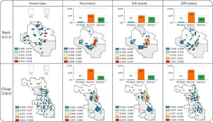
Heat maps illustrate the model predictions for Bogotá on November 16, 2018, and Chicago on June 3, 2022, considering 15% coverage area. These visualizations provide insights into potential data imbalances across the geographical groups under consideration. High-income areas are represented by white, while low-income areas are depicted in gray. Additionally, the maps highlight distinct variations in the adjusted data provided by the models. The naive and KDE models exhibit a higher spread of crime occurrence across areas than the SEPP model, where crime occurrences are more localized and less widespread
Figure 4 shows the Max-min and Gini metrics of PF (mean and 95% of confidence interval) versus different percentages of patrol coverage areas for each predictive model. This figure considers all different daily predictions resulting from the sliding window. As observed, the assignation of benefits to \(G_1\) and \(G_2\) have minor differences in Bogotá and Chicago, as evidenced by the Max-min plots. In Bogotá, when the results are rescaled to 100 events to improve interpretability (y-axis in Max-min plots), the discrepancy ranges from 0.25 to 1.5 error events between, regardless of the model used. In Chicago, the differences are even smaller, ranging from 0.2 to 0.8 error events. This evidence suggests that all predictive models exhibit minor average error differences (less than two events) between the groups relative to the percentage of the area that can be controlled or patrolled in a real scenario, indicating impartiality in the predictive security models’ performance. Figure 4 also shows the Gini’s PF metric plots. In this case, in Bogotá, the average fairness metric ranged between 5% and 20%, and for Chicago, between 4% and 10%. Which also suggests a similar benefit distribution among the groups. In this case, the KDE and naive plots resulted in similar PF values, as observed in Fig. 3, a persistent trend in Chicago.
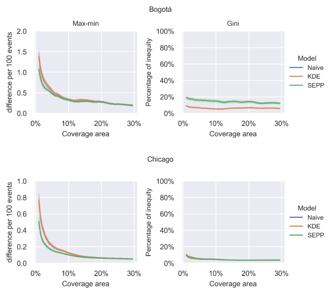
Max-min and Gini metrics for fairness evaluation in Bogotá and Chicago. Each point along the X-axis represents the percentage of area analyzed in each group relative to the total predictions. Along the Y-axis, the Max-min metric represents the disparity in benefits, while the Gini metric represents the percentage of this benefit disparity. These metrics are depicted for each model under evaluation
Figure 5 reports the RAF computed as the precision of classifications (patrol and non-patrol) for different patrol coverage areas between groups (\(G_1\) blue and \(G_2\) orange) in each model (columns). This figure also considers the full set of daily predictions resulting from the sliding window. As expected, when the percentage of area coverage increases, the patrolling success performance decreases for all models, i.e., the higher the patrolling area, the harder the patrolling task. Nevertheless, as observed, \(G_2\) consistently exhibits lower performance in the patrolling task than \(G_1\), indicating a better patrolling resource assignment for \(G_1\). In the case of Bogotá, when small coverage areas are considered, the gaps between average patrolling performances are small for native and KDE models. However, this gap increases when the percentage of coverage is lower, reaching a maximum difference between the means of groups of \(13\%\) for Bogotá and \(45\%\) for Chicago, an average of these differences of \(7\%\) for Bogotá and \(16\%\) for Chicago. Interestingly, Chicago’s patrolling performance values are higher than Bogotá, indicating better adjustments of the explored models in the former city. However, the gaps between average performances between spatial groups are also higher in Chicago than in Bogotá.
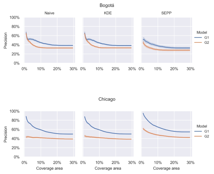
Trend of classification precision for patrolled and non-patrolled areas across a specific percentage range of the total coverage area (1% to 30%, simulating real scenarios) in each model for \(G_1\) and \(G_2\) from predictions in Chicago and Bogotá
3.2 Unfairness considering the full crime intensity
Figure 6 shows the performance of each model in Bogotá and Chicago based on the EMD metric. Complementary to the PF and RAF, this measure provides information about possible differences considering each spatial group’s complete crime intensity map without applying the thresholding. These distributions resulted from computing the EMD on the set of predictions from the sliding window, renormalizing each spatial group’s predicted crime intensity to sum one. In this case, the SEPP model was the top performer in both cities, as evidenced by its lower average EMD values: 0.005 for both \(G_1, G_2\) in Bogotá and 0.002, 0.003 respectively \(G_1, G_2\) in Chicago, suggesting that the SEPP model provides a more accurate prediction of the whole event distribution compared to the naive and KDE models. However, this figure also evidenced that predictive performances differ between groups when considering the full crime intensity map, privileging particular groups depending on the city.
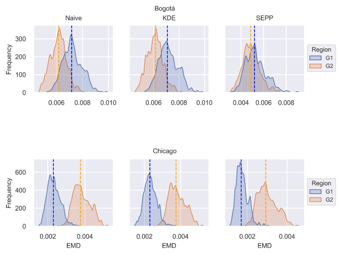
Visualization of the Earth Mover’s Distance (EMD) distribution computed for three predictive models—naive, KDE, and SEPP, grouped by \(G_1\) \(G_2\), for Bogotá and Chicago
The differences in performance between models may appear subtle at first glance. Still, they suggest that the naive and KDE models might need to capture the location and intensity of crime events more accurately than the SEPP model. This inference is strengthened by the observed discrepancies, as shown in Fig. 3. This trend is particularly evident in Chicago, where the results ranked low to high in KDE, naive, and SEPP, respectively. These performance differences can influence the PF result in the Max-min metric across coverage percentages, as shown in Fig. 4. However, it is worth noting to note that these values would be too low to indicate partiality in the models.
This performance model’s discrepancies also highlight the importance of precision in classifications of patrolling cells, as further emphasized Fig. 5, where the SEPP model resulted in the highest performance in RAF, suggesting that while the naive and KDE models may have particular strengths, such as computational simplicity or flexibility, they may need help to achieve the same level of accuracy and fairness as the SEPP model in predicting and allocating resources effectively.
3.3 Biases in data across groups
Figure 7 shows the histogram of total event counts for each day in the training data for each city. This result would provide insights into possible sources of bias influencing the predicted crime intensity maps (Flynn et al. 2022). As observed, there is a disparity in the distribution of reported events between \(G_1\) and \(G_2\). In Bogotá, this difference ranges from approximately 1 to 10 events between the two groups, while in Chicago, the gap is between 20 and 100 events. The partiality may result from an imbalance in reporting areas, recognized as a potential source of unfairness (Flynn et al. 2022). This reporting bias would influence results for RAF, which suggests a bias in the output models towards resource allocations. Notably, this bias is more evident in geographical areas characterized by low income, as observed in Bogotá and Chicago.
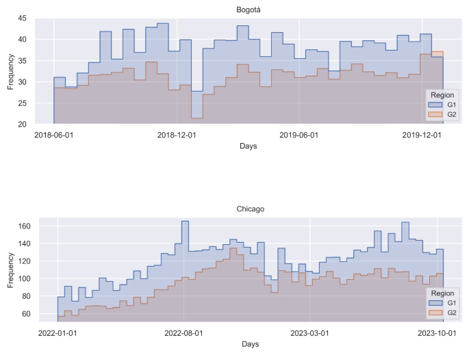
Disparity in event frequency within the training dataset for Bogotá and Chicago, revealing that \(G_2\), encompassing low-income areas, exhibits a lower event frequency compared to \(G_1\), representing high-income areas
3.4 Economic activity and predictive bias
Figure 8 presents heat maps of the data used to train and test the models and shows the distribution of enterprise locations and central business districts for both Bogotá and Chicago. These maps provide visual evidence of the heterogeneity of spatial data that may contribute to observed predictive disparities.
As shown in Fig. 8, in both Chicago and Bogotá, most of the business activity and company operations are concentrated within the \(G_1\) region. Interestingly, in Bogotá, the hotspot appears to be located along the border between \(G_1\) and \(G_2\), with the economic centers primarily located in \(G_1\), adjacent to \(G_2\). This spatial concentration of commercial activity is significant, as previous research suggests that regions with greater economic infrastructure tend to exhibit higher rates of reported crime events, not necessarily due to increased criminality but rather due to higher surveillance, policing presence, and reporting propensity (Rotaru et al. 2021; Akpinar et al. 2021).
The alignment between the enterprise zones and the group regions can partly explain the disparities observed in RAF and PF in \(G_1\) and \(G_2\). In Chicago, where economic activity is concentrated \(G_1\), the models tend to allocate more patrol resources to this group, reinforcing the disparities noted in Sections 3.1 and 3.2. In contrast, in Bogotá, the proximity of business areas to the boundary between \(G_1\) and \(G_2\) creates a more complex spatial interaction.
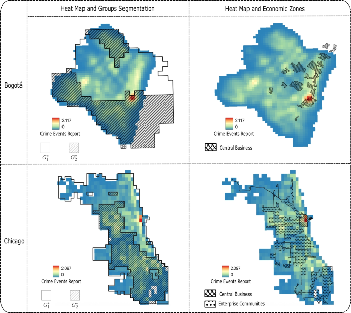
Heat maps illustrate data used for the models. The maps reveal crime hotspots concentrated in specific urban zones that spatially align with the central business and commercial districts of both Bogotá and Chicago. In Chicago, these hotspots are entirely contained within the region \(G_1\), while in Bogotá, they are primarily located in region \(G_1\), adjacent to \(G_2\)
4 Discussion
Predictive policing uses data-driven models to forecast criminal activities and inform law enforcement strategies. However, concerns about algorithmic fairness have emerged, as these models can reinforce discrimination and inequalities, especially among vulnerable populations. This study proposes a framework to quantify the fairness of predictive security models by examining their capacity to distribute benefits impartially through prediction and resource allocation.
Algorithmic fairness aims to understand and mitigate biases in machine learning models (Wang et al. 2023). Fairness is typically quantified by comparing the distribution of benefits provided by predictive models among different sub-populations using equity metrics (Wang et al. 2023). A model is fair when it ensures equitable treatment across various groups (Wang et al. 2023; Caton and Haas 2024). Most fairness quantification strategies focus on individual-focused predictive systems (Mittelstadt et al. 2023).
Assessing fairness in spatially-based predictive models requires further investigation (Hardyns and Rummens 2018; Flynn et al. 2022). Our results (see Figs. 4, 5) indicate that key concepts of algorithmic fairness, such as benefit functions and fairness metrics, can be applied to spatially-based characterizations. Spatial predictions are used in fields like environmental science, urban planning, agriculture, disaster management, and health (Jiang 2019; Khan 2019; Melo et al. 2020; Fayet et al. 2020). Therefore, our framework for spatially-based fairness metrics can help quantify how demographic or socioeconomic characteristics influence predictions and decisions in these fiel
Unfair predictive models can perpetuate inequalities and stigmatize certain areas or groups in predictive security systems (Flynn et al. 2022). For example, biases in crime prediction models trained with skewed data can reinforce existing discriminations and inequalities (Flynn et al. 2022; Dass et al. 2023). Our results show these biases also exist in spatially-based prediction systems, affecting resource allocation for crime prevention (see Fig. 5). This evidence suggests another source of unfairness related to resource allocation, which merits further exploration.
Fairness in resource allocation is increasingly recognized across domains such as healthcare, finance, and law enforcement (Hardt et al. 2016; Flores et al. 2016; Hernandez-Boussard et al. 2023). For instance, fairness in patrolling should be based on objective risk assessments rather than biases (Kleinberg et al. 2016; Selbst et al. 2019). Our results suggest that measuring fairness in resource allocation can be achieved for spatially-based models in predictive security systems. Our proposed framework quantifies both predictive and resource allocation fairness. While most existing studies focus on the unequal distribution of benefits in prediction outputs, our approach also assesses how predictions influence resource allocation in tasks like patrol assignments. This dual measure provides a comprehensive view of the impact of prediction systems on populations. Future work should explore the impact of more sophisticated allocation strategies on fairness (Wheeler 2018).
While our framework quantifies fairness across different predictive policing models and resource allocation strategies, this work is not focuses on a key practical and ethical challenge: the widely discussed trade-off between fairness and effectiveness (Kleinberg et al. 2016; Corbett-Davies et al. 2018; Mitchell et al. 2021; Mittelstadt et al. 2023). This tension arises because optimizing predictive models solely for overall crime reduction efficiency, by focusing resources on areas where prediction is easiest or crime incidence is historically highest, can inadvertently exacerbate disparities across different geographic or demographic groups. Improving fairness, conversely, often requires reallocating resources or adjusting predictions in ways that may not maximize overall crime prevention efficiency, potentially leading to a slight reduction in effectiveness (Elzayn et al. 2018; Lahoti et al. 2019). This conflict between maximizing utility and ensuring equitable outcomes is a central debate in the deployment of AI in public safety (Liberatore et al. 2022, 2023).
Crime modeling pipelines typically involve steps like data collection and processing, predictive modeling (forecasting crime events), and subsequent resource allocation (dispatching police) (Mikołajczyk-Bareła and Grochowski 2023; Ravishankar et al. 2023). Interestingly, our findings reveal a notable disparity between fairness at the prediction stage (Fig. 4), where models appear relatively fair, and fairness at the resource allocation stage (Fig. 5), where significant spatial disparities emerge. This suggests that fairness properties do not necessarily propagate linearly through the pipeline; a fair prediction does not guarantee fair resource allocation. This observation raises a fundamental research question: how does fairness or unfairness from one stage of a predictive policing pipeline affect the fairness of subsequent stages? Understanding this “fairness propagation” is crucial for designing interventions that ensure equitable outcomes throughout the entire system, from data collection biases to resource deployment.
Furthermore, our analysis suggests that the spatial distribution of economic activity influences reported crime patterns and predictability across urban areas (Rotaru et al. 2021; Akpinar et al. 2021), potentially concentrating predictable crime in areas with high business density (Fig. 8). These variations in inherent predictability and reporting rates across space add another layer of complexity to the fairness-effectiveness trade-off. They imply that disparities in fairness metrics may stem not only from model design but also from structural inequalities reflected in the data itself. Nevertheless, the societal consequences of such disparities, including potential over-policing in easily predictable areas or under-servicing in less predictable ones (Liberatore et al. 2022, 2023). While our current study focuses on quantifying existing disparities rather than optimizing this balance, future research building upon our framework should explore methods for incorporating socioeconomic or other contextual covariates into predictive models.
Evaluating fairness in predictive systems relies on how groups are defined, whether by demographic attributes (for instance, race, gender, and income) (Wheeler 2018; Wang et al. 2023) wich give us the spatial divisions of \(G_1\)/\(G_2\) segmentation. Group-based fairness metrics are sensitive to these definitions, as group boundaries (or threshold segmentation) directly shape evaluation outcomes and perceptions of equity (Barocas et al. 2023). Using broad spatial segmentations, especially those reflecting socioeconomic divides, presents a challenge: they generalize finer-grained disparities within or across subregions (Mitchell et al. 2021; Flynn et al. 2022; Dass et al. 2023), especially when treating a large zone. Our framework uses a binary spatial segmentation to illustrate key fairness dynamics, and future work should examine fairness across alternative, multi-scale spatial partitions reflecting socioeconomic and demographic heterogeneity.
This study has limitations. It only explores three predictive security models and uses a particular configuration for daily predictions. Future research should investigate other models and configurations, such as long-term predictions for urban planning (Koutra and Ioakimidis 2022). Additionally, only two segmentation areas were used, limiting model comparison. By examining the overall performance of predictive models and their fairness in achieving specific objectives, stakeholders can ensure these tools contribute to equitable outcomes and effectively address systemic biases. Further research is warranted to refine fairness assessment methodologies and enhance the equity of predictive modeling practices.
Notes
Data available at
Last accessed May 22, 2025:
Last accessed May 22, 2025:
References
Abu-Mostafa YS, Magdon-Ismail M, Lin HT (2012) Learning from data. AMLBook, S.l
Google Scholar
Akpinar NJ, De-Arteaga M, Chouldechova A (2021) The effect of differential victim crime reporting on predictive policing systems. In: Proceedings of the 2021 ACM conference on fairness, accountability, and transparency, ACM, Virtual Event Canada. pp 838–849.
Alikhademi K, Drobina E, Prioleau D, Richardson B, Purves D, Gilbert JE (2022) A review of predictive policing from the perspective of fairness. Artif Intell Law 30:1–17.
Article
Google Scholar
Barocas S, Hardt M, Narayanan A (2023) Fairness and machine learning: limitations and opportunities. MIT Press
Benbouzid B (2019) To predict and to manage. Predictive policing in the United States. Big Data Soc 6:2053951719861703.
Article
Google Scholar
Bureau UC (2014) Census data - selected socioeconomic indicators in Chicago, 2008–2012: City of Chicago: data portal.
Caton S, Haas C (2024) Fairness in machine learning: a survey. ACM Comput Surv 56:1–38.
Article
Google Scholar
Cheng T, Chen T (2021) Urban crime and security. In: Shi W, Goodchild MF, Batty M, Kwan MP, Zhang A (Eds) Urban informatics. Springer, Singapore, pp 213–228.
Ciotti M, Ciccozzi M, Terrinoni A, Jiang WC, Wang CB, Bernardini S (2020) The COVID-19 pandemic. Crit Rev Clin Lab Sci 57:365–388.
Article
Google Scholar
Corbett-Davies S, Gaebler JD, Nilforoshan H, Shroff R, Goel S (2018) The measure and mismeasure of fairness.
Dass RK, Petersen N, Omori M, Lave TR, Visser U (2023) Detecting racial inequalities in criminal justice: towards an equitable deep learning approach for generating and interpreting racial categories using mugshots. AI Soc 38:897–918.
Article
Google Scholar
Department CP (2024) Crimes - 2001 to present: City of Chicago: Data portal.
Dimas Hoyos DL, Ana María VM, Anyela María GA (2015) Teusaquillo, con la mejor calidad de vida en Bogotá.
Elzayn H, Jabbari S, Jung C, Kearns M, Neel S, Roth A, Schutzman Z (2018) Fair algorithms for learning in allocation problems.
Fayet Y, Praud D, Fervers B, Ray-Coquard I, Blay JY, Ducimetiere F, Fagherazzi G, Faure E (2020) Beyond the map: evidencing the spatial dimension of health inequalities. Int J Health Geogr 19:46.
Article
Google Scholar
Flores AW, Bechtel K, Lowenkamp CT (2016) False positives, false negatives, and false analyses: a rejoinder to machine bias: There’s software used across the country to predict future criminals. and it’s biased against blacks. Federal Probation Journal.
Flynn C, Guha A, Majumdar S, Srivastava D, Zhou Z (2022) Towards algorithmic fairness in space-time: filling in black holes.
Hardt M, Price E, Srebro N (2016) Equality of opportunity in supervised learning.
Hardyns W, Rummens A (2018) Predictive policing as a new tool for law enforcement? Recent developments and challenges. Eur J Crim Policy Res 24:201–218.
Article
Google Scholar
Hernandez-Boussard T, Siddique SM, Bierman AS, Hightower M, Burstin H (2023) Promoting equity in clinical decision making: dismantling race-based medicine. Health Affairs (Project Hope) 42:1369–1373.
Article
Google Scholar
Hung TW, Yen CP (2023) Predictive policing and algorithmic fairness. Synthese 201:206.
Article
Google Scholar
Jiang Z (2019) A Survey on Spatial Prediction Methods. IEEE Trans Knowl Data Eng 31:1645–1664.
Jonathan Levy Cc (2025) Central_business_district | City of Chicago | Data Portal.
Joshi C, Curtis-Ham S, D’Ath C, Searle D (2021) Considerations for developing predictive spatial models of crime and new methods for measuring their accuracy. ISPRS Int J Geo Inf 10:597.
Khan KE (2019) Decoding urban inequality : the applications of machine learning for mapping inequality in cities of the Global South. Thesis. Massachusetts Institute of Technology.
Kingi H, Zhang C, Gasperini B, Heuser A, Huynh M, Moore J (2018) An assessment of crime forecasting models. In: Proceedings of the FCSM research and policy conference, federal committee on statistical methodology, Washington, DC. Presented in March 2018
Kleinberg J, Mullainathan S, Raghavan M (2016) Inherent trade-offs in the fair determination of risk scores.
Koutra S, Ioakimidis CS (2022) Unveiling the potential of machine learning applications in urban planning challenges. Land 12:83.
Lahoti P, Gummadi KP, Weikum G (2019) Operationalizing individual fairness with pairwise fair representations. Proc VLDB Endow 13:506–518.
Article
Google Scholar
Lavrakas PJ, Skogan WG (1984) Citizen participation and community crime prevention, 1979: Chicago metropolitan area survey: archival version.
Lee J, Gong J, Li S (2017) Exploring spatiotemporal clusters based on extended kernel estimation methods. Int J Geogr Inf Sci 31:1154–1177.
Article
Google Scholar
Liberatore F, Camacho-Collados M, Quijano-Sánchez L (2022) Equity in the police districting problem: balancing territorial and racial fairness in patrolling operations. J Quant Criminol 38:1–25.
Article
Google Scholar
Liberatore F, Camacho-Collados M, Quijano-Sánchez L (2023) Towards social fairness in smart policing: Leveraging territorial, racial, and workload fairness in the police districting problem. Socioecon Plann Sci 87:101556.
Manning M, Wong GTW, Graham T, Ranbaduge T, Christen P, Taylor K, Wortley R, Makkai T, Skorich P (2018) Towards a ‘smart’ cost-benefit tool: using machine learning to predict the costs of criminal justice policy interventions. Crime Sci 7:12.
Article
Google Scholar
Melo SN, Boivin R, Morselli C (2020) Spatial dark figures of rapes: (In)Consistencies across police and hospital data. J Environ Psychol 68:101393.
Mikołajczyk-Bareła A, Grochowski M (2023) A survey on bias in machine learning research. arXiv:2308.11254
Mitchell S, Potash E, Barocas S, D’Amour A, Lum K (2021) Algorithmic fairness: choices, assumptions, and definitions. Ann Rev Stat Its Appl 8:141–163.
Article
MathSciNet
Google Scholar
Mittelstadt B, Wachter S, Russell C (2023) The unfairness of fair machine learning: levelling down and strict egalitarianism by default.
Mohler GO, Short MB, Brantingham PJ, Schoenberg FP, Tita GE (2011) Self-exciting point process modeling of crime. J Am Stat Assoc 106:100–108.
Article
MathSciNet
Google Scholar
Morenoff JD, Sampson RJ, Raudenbush SW (2001) Neighborhood inequality, collective efficacy, and the spatial dynamics of urban violence. Criminology 39:517–558.
Article
Google Scholar
Muggah R, Tobón KA (2019) Reducing Latin America’s violent hot spots. Aggress Violent Beh 47:253–256.
Rajadurai S, Ah SHBAB, Zainol RB, Azman ZB (2022) Crime prevention through environmental design and its challenges in reducing crime: a case of Selangor, Malaysia. Secur J 35:934–947.
Article
Google Scholar
Ravishankar P, Mo Q, McFowland E, Neill DB (2023) Provable detection of propagating sampling bias in prediction models.
Rene Guarin Cortes IDdT (2025) Zonas Interés Turístico. Bogotá D.C. - Datos Abiertos Bogotá.
Rosser G, Cheng T (2019) Improving the robustness and accuracy of crime prediction with the self-exciting point process through isotropic triggering. Appl Spat Anal Policy 12:5–25.
Article
Google Scholar
Rotaru V, Huang Y, Li T, Evans J, Chattopadhyay I (2021) Precise event-level prediction of urban crime reveals signature of enforcement bias.
Rubner Y, Tomasi C, Guibas LJ (2000) The earth mover’s distance as a metric for image retrieval. Int J Comput Vision 40:99–121.
Article
Google Scholar
Sacharidis D, Giannopoulos G, Papastefanatos G, Stefanidis K (2023) Auditing for spatial fairness.
Selbst AD, Boyd D, Friedler SA, Venkatasubramanian S, Vertesi J (2019) Fairness and abstraction in sociotechnical systems. In: Proceedings of the conference on fairness, accountability, and transparency, ACM, Atlanta GA USA. pp 59–68.
Sherman LW, Weisburd D (1995) General deterrent effects of police patrol in crime “hot spots’’: A randomized, controlled trial. Justice Q 12:625–648.
Article
Google Scholar
Sriram K, Gupta D, Parikh R (2024) Movement of insurgent gangs: A Bayesian kernel density model for incomplete temporal data. doi: 550/ARXIV.2401.01231
Villegas AJR, Nungo JS, Tobon LG, Rubio MD, Gomez F (2023) Modelling underreported spatio-temporal crime events. PLoS ONE 18:e0287776.
Article
Google Scholar
Wang Y, Ma W, Zhang M, Liu Y, Ma S (2023) A survey on the fairness of recommender systems. ACM Trans Inf Syst 41:1–43.
Article
Google Scholar
Wheeler A (2018) Creating optimal patrol areas using the p-median model.
Wu J, Abrar SM, Awasthi N, Frías-Martínez V (2023) Auditing the fairness of place-based crime prediction models implemented with deep learning approaches. Comput Environ Urban Syst 102:101967.
Xie Y, He E, Jia X, Chen W, Skakun S, Bao H, Jiang Z, Ghosh R, Ravirathinam P (2022) Fairness by “Where’’: a statistically-robust and model-agnostic bi-level learning framework. Proc AAAI Conf Artif Intell 36:12208–12216.
Article
Google Scholar
Zambom AZ, Dias R (2012) A review of kernel density estimation with applications to econometrics.
Zhu R, Aqlan F, Yang H (2022) Optimal resource allocation for coverage control of city crimes. In: Yang H, Qiu R, Chen W (eds) AI and analytics for public health, Springer International Publishing, Cham. pp 149–161
Download references
Acknowledgements
We thank the project Diseño y validación de modelos de analítica predictiva de fenómenos de seguridad convivencia para la toma de decisiones en Bogotá (BPIN: 2016000100036) for kindly providing the data.
Funding
Open Access funding provided by Colombia Consortium
Author information
Ethics declarations
Conflicts of Interest
All authors declare no potential, perceived, or real conflict of interest regarding the content of this paper.
Additional information
Publisher's Note
Springer Nature remains neutral with regard to jurisdictional claims in published maps and institutional affiliations.
Rights and permissions
Open Access This article is licensed under a Creative Commons Attribution 4.0 International License, which permits use, sharing, adaptation, distribution and reproduction in any medium or format, as long as you give appropriate credit to the original author(s) and the source, provide a link to the Creative Commons licence, and indicate if changes were made. The images or other third party material in this article are included in the article’s Creative Commons licence, unless indicated otherwise in a credit line to the material. If material is not included in the article’s Creative Commons licence and your intended use is not permitted by statutory regulation or exceeds the permitted use, you will need to obtain permission directly from the copyright holder. To view a copy of this licence, visit
Reprints and permissions
About this article
Cite this article
Hernández, D., Pulido, C. & Gómez, F. Quantifying fairness in spatial predictive policing.
Artif Intell Law (2026).
Download citation
Received:
Accepted:
Published:
Version of record:


